Distinguish White Wines From Red Wines
Perform EDA on Red & White Wine Means:
I conducted an exploratory data analysis in comparing means for the 11 chemical attributes in the red and white wines. Notably, ‘totalSulfurDioxide’ showed significant mean differences, followed by ‘freeSulfurDioxide’ and ‘residualSugar.’ These attributes currently stand out showing a clear difference between the means of white and red wines.
Perform MANOVA to determine if there are a significant difference in mean vectors between red and white wines with a 95% confidence level.
\begin{align*} &H_0: \bar{\mu}_{\text{red}} = \bar{\mu}_{\text{white}} \\ &H_A: \bar{\mu}_{\text{red}} \neq \bar{\mu}_{\text{white}} \end{align*}
MANOVA Results
The MANOVA reveals a significant disparity in the means for specific chemical traits between red and white wines. Notably, Pillai’s Trace (0.86158) indicates a robust effect, accounting for approximately 86.128\% of the variance. The p-value of 2.2 \times 10^{-16} signifies significant differences in the mean vectors. Hence, the MANOVA decisively rejects the null hypothesis of no difference in means, and we have exceptionally high confidence in accepting the alternative-that there is a difference in means between each wine.
Perform Classification Modeling on Red & White Wines
Train-Test Split & Cross-Validation Set up
I performed a train-test split to ensure the models can handle new, unseen data. I allocated 70\% to the training data to have a larger sample for the testing data (30\%). To enhance reliability, I employed cross-validation, repeatedly splitting the data into different training and testing sets. This approach provides a more comprehensive evaluation of the model’s effectiveness.
Random Forest, SVM and Logistic Models
For my models, I’ve selected Random Forest, Support Vector Machine, and Logistic Regression as promising candidates for effective classification. Logistic Regression is particularly beneficial in binary classification scenarios due to its simplicity and interpretability. Meanwhile, Random Forest excels in capturing complex relationships through ensemble learning, and Support Vector Machine demonstrates proficiency in handling both linear and non-linear patterns. As the results will show later, Random Forest performed the best followed by SVM. Note, the models were not tuned to use their best hyperparameters.
Metrics & Variable Importance
The confusion matrix for the red and white wine classification using the Random Forest model shows strong performance. The model correctly identified 474 red wines and 1464 white wines, with only 5 red wines and 5 white wines misclassified. This indicates high accuracy in both precision and recall. In comparison to the Support Vector Machine (SVM) and Logistic Regression models, the Random Forest performed better by minimizing misclassifications. The SVM model had slightly more misclassified instances (13 in total), while the Logistic Regression model had 17 misclassifications. The Random Forest’s performance makes it a better choice for this classifying red and white wines compared to SVM and Logistic Regression.
The variable importance analysis shows that “chlorides,” with a significance of 100%, is the most crucial feature for distinguishing red and white wines. Additionally, “totalSulfurDioxide” (96.92%) and “volatileAcidity” (43.47%) also played key roles, contributing to the model’s clear performance in wine classification.
Classifying a New Red Wine Drawn From The Same Population
To estimate the probability of correctly classifying a new red wine drawn from the same population, we can use the concept of recall.
In our confusion matrix:
\text{Recall (for red wine)} = \frac{\text{True Positives (TP)}}{\text{True Positives (TP) + False Negatives (FN)}}
To find the probability:
\text{Recall (for red wine)} = \frac{474}{474 + 5} = \frac{474}{479} = 0.9896
So, the estimated probability of correctly classifying a new red wine, drawn from the same population, is approximately \frac{474}{479}, or roughly 98.96\%. This suggests a very high probability of correctly identifying red wines based on the model’s current performance.
K-Means Clustering
I chose k-means clustering with Euclidean distance for its efficiency with standardized numerical data. While k = 2 visually showed a clear distinction between red and white wines, higher k values (for example, 3 or 4) led to overlapping clusters, affecting the meaningful separation observed with k = 2.
Which Variables Are The Most Important To Wine Quality In Red Wines?
Perform MANOVAs To Determine If There Are A Significant Difference In Mean Vectors Between Wines With Different Quality/Quality Groups With A 95% Confidence Level.
MANOVA for Quality Levels 3, 4, 5, 6, 7, 8
\begin{align*} &H_0: \mu_2 = \mu_3 = \mu_4 = \mu_5 = \mu_6 = \mu_7 = \mu_8 \\ &H_A: \text{At least one of } \mu_2, \mu_3, \mu_4, \mu_5, \mu_6, \mu_7, \text{ or } \mu_8 \text{ is different} \end{align*}
In the first analysis, we looked at the Original Quality Scores, and the results were highly significant. The p-value was super close to zero, less than 2.2 x 10^{-16}. This means there are big differences in the average chemical properties for different quality scores. Therefore, the mean vectors for each quality level varied, providing strong support for rejecting the null hypothesis.
MANOVA for Quality Groups [Low, Medium, High]
\begin{align*} &H_0: \mu_{\text{Low}} = \mu_{\text{Medium}} = \mu_{\text{High}} \\ &H_A: \text{At least one of } \mu_{\text{Low}}, \mu_{\text{Medium}}, \text{ or } \mu_{\text{High}} \text{ is different} \end{align*}
In the second analysis, we focused on Quality Groups (Low, Medium, High), and the results were also highly significant. The p-value was very close to zero, less than 2.2 x 10^{-16}. This indicates significant differences in the average chemical properties across different quality groups. We have strong evidence that the mean vectors between each quality group differed. Therefore, we have evidence to reject the null and be in favor of the alternative.
Overall MANOVA Test Conclusion
To summarize, our MANOVA tests reveal significant differences in average values for both original quality scores and quality groups. For original scores, statistics like Pillai’s trace and Wilks’ lambda had extremely low p-values p < 2.2 x 10^{-16}. Quality groups exhibited similar results.
Perform Classification on Quality for Red Wines
Random Forest and SVM models
I performed the same procedure from the previous classification of red and white wines. I’ve selected Random Forest & Support Vector Machine the top models for classification. Logistic Regression is not designed for multiple classes. Interestingly, the Random Forest performed the best again, followed by SVM. It’s important to note that the models were not fine-tuned for hyperparameters at this stage.
Metrics & Variable Importance
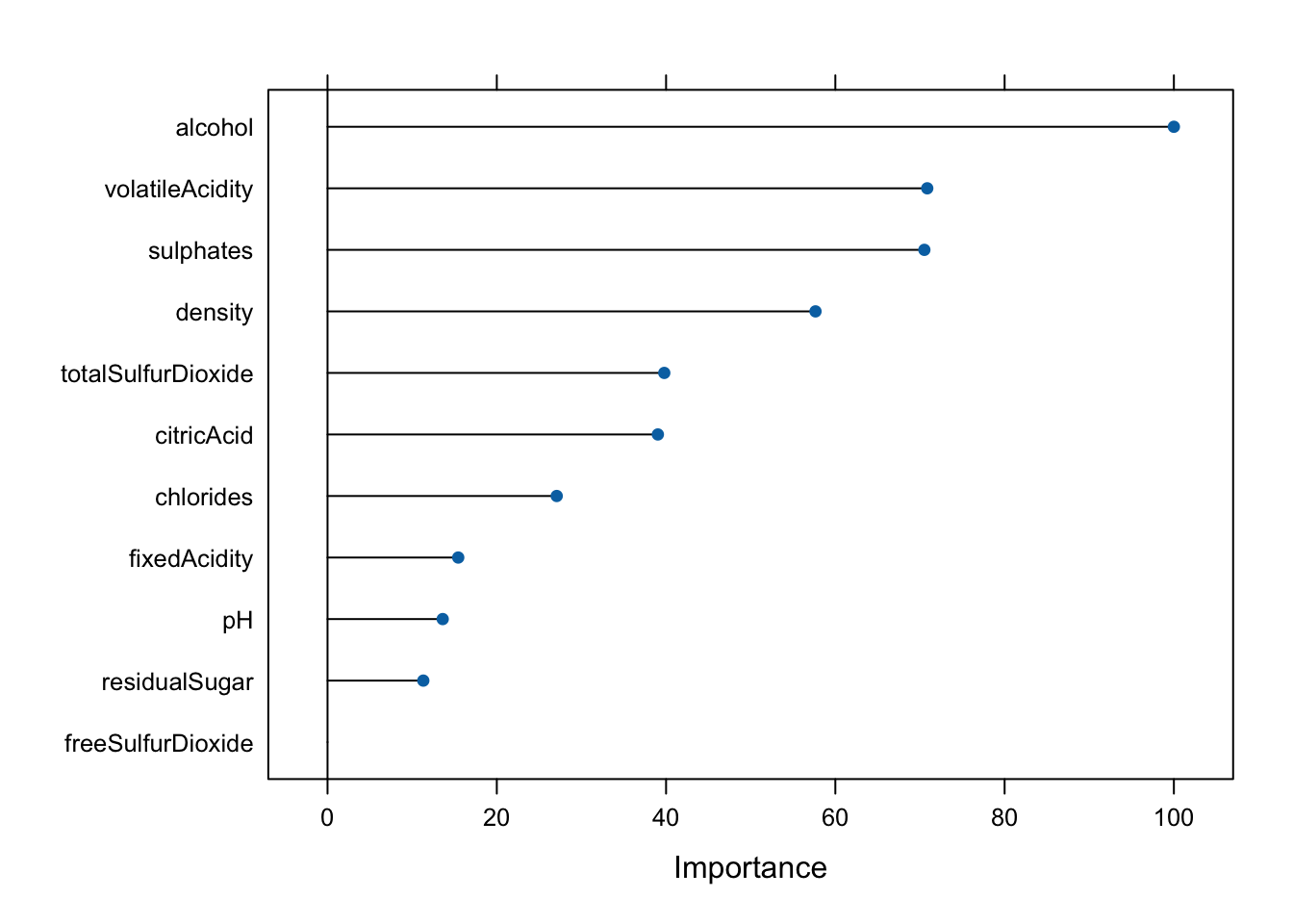
Random Forest emerged as the top-performing model once again, with an accuracy of 69.2\%. For instance, we can observe that quality level 5 has the highest number of correct predictions (163), while quality levels 4 and 6 have some misclassifications. Among the features, alcohol, total sulfur dioxide, and volatile acidity emerged as the top three influential variables, showcasing their significance in predicting wine quality in red wines.
Perform Principal Component Analysis
Explaining PC1 & PC2
PC1 can be interpreted as representing “Wine Body.” Red wines with higher fixed acidity, citric acid, free sulfur dioxide, and total sulfur dioxide contribute positively to this component, indicating a fuller and more robust body. Hence, higher levels of volatile acidity, residual sugar, and alcohol contribute negatively to this component.
PC2 can be labeled as “Fermentation Characteristics.” Additionally, red wines with elevated levels of free sulfur dioxide, total sulfur dioxide, and density contribute positively to this component, highlighting aspects related to the fermentation process. On the other end, higher alcohol content and volatile acidity contribute negatively to PC2.
Random Forest Model with 2 PCA
In the confusion matrix, it’s evident that the model struggled to accurately predict certain classes, particularly in categories 3, 4, and 7, where the predicted values differ from the actual values. To add, random forest model achieved an accuracy of 58.07% which is quite below the previous models. Despite its limitations, the model demonstrated some success in capturing patterns related to “Wine Body” and “Fermentation Characteristics.” And it’s with just 2 variables with linear combinations.
Random Forest Model with 11 PCAs
The random forest model attained an accuracy of 68.13%. Plus, it excelled in predicting class 5 but faced challenges in classes 3, 4, 6, and 7. Principal Component Analysis (PCA) highlights PC2 as the most influential (100%), followed by PC3 (80.49%), PC5 (32.47%), and others. This suggests a need for further analysis to enhance predictions in specific classes and leverage insights from key Principal Components for optimization.
Comparison between Random Forest Models (normal, 2PCs, 11PCs)
In comparing the Random Forest models, both the normal model and the 11 PCs model achieve an accuracy of approximately 68%, surpassing the 2 PCs model, which attains an accuracy of 58.07%. It’s noteworthy that the 2 PCs model demonstrates the potency of PCA, albeit with a trade-off in interpretability. Despite the challenges encountered, each model variant provides valuable insights for optimizing the predictive power. The room for improvement is wide open. Factors such as hyperparameter tuning, other models that were not explored, feature engineering, and delving further into factor analysis are instances that could be used to maximize performance.
Appendix
Goal 1: Distinguish White Wines From Red Wines
# Set scipen to a high value to disable scientific notation
options(scipen = 999)
library(tidyverse)
library(caret)
library(cluster)
library(factoextra)
library(MASS)
library(rstatix)

# Read in the wine datasets
redWine <- read_csv("/data/winequality-red.csv")
whiteWine <- read_csv("/data/winequality-white.csv")

# Look at the structure of the wine data
glimpse(redWine)
Rows: 1,599
Columns: 12
$ `fixed acidity` <dbl> 7.4, 7.8, 7.8, 11.2, 7.4, 7.4, 7.9, 7.3, 7.8, 7…
$ `volatile acidity` <dbl> 0.700, 0.880, 0.760, 0.280, 0.700, 0.660, 0.600…
$ `citric acid` <dbl> 0.00, 0.00, 0.04, 0.56, 0.00, 0.00, 0.06, 0.00,…
$ `residual sugar` <dbl> 1.9, 2.6, 2.3, 1.9, 1.9, 1.8, 1.6, 1.2, 2.0, 6.…
$ chlorides <dbl> 0.076, 0.098, 0.092, 0.075, 0.076, 0.075, 0.069…
$ `free sulfur dioxide` <dbl> 11, 25, 15, 17, 11, 13, 15, 15, 9, 17, 15, 17, …
$ `total sulfur dioxide` <dbl> 34, 67, 54, 60, 34, 40, 59, 21, 18, 102, 65, 10…
$ density <dbl> 0.9978, 0.9968, 0.9970, 0.9980, 0.9978, 0.9978,…
$ pH <dbl> 3.51, 3.20, 3.26, 3.16, 3.51, 3.51, 3.30, 3.39,…
$ sulphates <dbl> 0.56, 0.68, 0.65, 0.58, 0.56, 0.56, 0.46, 0.47,…
$ alcohol <dbl> 9.4, 9.8, 9.8, 9.8, 9.4, 9.4, 9.4, 10.0, 9.5, 1…
$ quality <dbl> 5, 5, 5, 6, 5, 5, 5, 7, 7, 5, 5, 5, 5, 5, 5, 5,…glimpse(whiteWine)Rows: 4,898
Columns: 12
$ `fixed acidity` <dbl> 7.0, 6.3, 8.1, 7.2, 7.2, 8.1, 6.2, 7.0, 6.3, 8.…
$ `volatile acidity` <dbl> 0.27, 0.30, 0.28, 0.23, 0.23, 0.28, 0.32, 0.27,…
$ `citric acid` <dbl> 0.36, 0.34, 0.40, 0.32, 0.32, 0.40, 0.16, 0.36,…
$ `residual sugar` <dbl> 20.70, 1.60, 6.90, 8.50, 8.50, 6.90, 7.00, 20.7…
$ chlorides <dbl> 0.045, 0.049, 0.050, 0.058, 0.058, 0.050, 0.045…
$ `free sulfur dioxide` <dbl> 45, 14, 30, 47, 47, 30, 30, 45, 14, 28, 11, 17,…
$ `total sulfur dioxide` <dbl> 170, 132, 97, 186, 186, 97, 136, 170, 132, 129,…
$ density <dbl> 1.0010, 0.9940, 0.9951, 0.9956, 0.9956, 0.9951,…
$ pH <dbl> 3.00, 3.30, 3.26, 3.19, 3.19, 3.26, 3.18, 3.00,…
$ sulphates <dbl> 0.45, 0.49, 0.44, 0.40, 0.40, 0.44, 0.47, 0.45,…
$ alcohol <dbl> 8.8, 9.5, 10.1, 9.9, 9.9, 10.1, 9.6, 8.8, 9.5, …
$ quality <dbl> 6, 6, 6, 6, 6, 6, 6, 6, 6, 6, 5, 5, 5, 7, 5, 7,…# Run a quick summary for both datasets
#summary(redWine)
#summary(whiteWine)
# Add a 'wine_type' column to identify the wine type
redWine$wineType <- "red"
whiteWine$wineType <- "white"
# Combine the datasets
wine <- bind_rows(redWine, whiteWine)
# Rename columns for better readability and consistency
wine <- wine %>%
dplyr::mutate(fixedAcidity = `fixed acidity`,
volatileAcidity = `volatile acidity`,
citricAcid = `citric acid`,
residualSugar = `residual sugar`,
freeSulfurDioxide = `free sulfur dioxide`,
totalSulfurDioxide = `total sulfur dioxide`,
wineType = factor(wineType, levels = c("red", "white"))) %>%
dplyr::select(-c(`fixed acidity`,
`volatile acidity`,
`citric acid`,
`residual sugar`,
`free sulfur dioxide`,
`total sulfur dioxide`))
# Check for quality counts
wine %>%
group_by(quality) %>%
summarise(totalCount = n())# A tibble: 7 × 2
quality totalCount
<dbl> <int>
1 3 30
2 4 216
3 5 2138
4 6 2836
5 7 1079
6 8 193
7 9 5wineDs <- wine %>%
select(-quality)
names(wineDs) [1] "chlorides" "density" "pH"
[4] "sulphates" "alcohol" "wineType"
[7] "fixedAcidity" "volatileAcidity" "citricAcid"
[10] "residualSugar" "freeSulfurDioxide" "totalSulfurDioxide"glimpse(wineDs)Rows: 6,497
Columns: 12
$ chlorides <dbl> 0.076, 0.098, 0.092, 0.075, 0.076, 0.075, 0.069, 0.…
$ density <dbl> 0.9978, 0.9968, 0.9970, 0.9980, 0.9978, 0.9978, 0.9…
$ pH <dbl> 3.51, 3.20, 3.26, 3.16, 3.51, 3.51, 3.30, 3.39, 3.3…
$ sulphates <dbl> 0.56, 0.68, 0.65, 0.58, 0.56, 0.56, 0.46, 0.47, 0.5…
$ alcohol <dbl> 9.4, 9.8, 9.8, 9.8, 9.4, 9.4, 9.4, 10.0, 9.5, 10.5,…
$ wineType <fct> red, red, red, red, red, red, red, red, red, red, r…
$ fixedAcidity <dbl> 7.4, 7.8, 7.8, 11.2, 7.4, 7.4, 7.9, 7.3, 7.8, 7.5, …
$ volatileAcidity <dbl> 0.700, 0.880, 0.760, 0.280, 0.700, 0.660, 0.600, 0.…
$ citricAcid <dbl> 0.00, 0.00, 0.04, 0.56, 0.00, 0.00, 0.06, 0.00, 0.0…
$ residualSugar <dbl> 1.9, 2.6, 2.3, 1.9, 1.9, 1.8, 1.6, 1.2, 2.0, 6.1, 1…
$ freeSulfurDioxide <dbl> 11, 25, 15, 17, 11, 13, 15, 15, 9, 17, 15, 17, 16, …
$ totalSulfurDioxide <dbl> 34, 67, 54, 60, 34, 40, 59, 21, 18, 102, 65, 102, 5…sum(is.na(wineDs))[1] 0Perform EDA on Red & White Wine Means:
# Calculate the mean vectors for red and white wines
# separately for each of the 11 chemical attributes
meanVectors <- wineDs %>%
  group_by(wineType) %>%
  summarize_all(mean)

# Display the mean vectors
head(meanVectors, 2)
# A tibble: 2 × 12
wineType chlorides density pH sulphates alcohol fixedAcidity
<fct> <dbl> <dbl> <dbl> <dbl> <dbl> <dbl>
1 red 0.0875 0.997 3.31 0.658 10.4 8.32
2 white 0.0458 0.994 3.19 0.490 10.5 6.85
# ℹ 5 more variables: volatileAcidity <dbl>, citricAcid <dbl>,
# residualSugar <dbl>, freeSulfurDioxide <dbl>, totalSulfurDioxide <dbl># Convert to long format for plotting
meanDs <- tidyr::gather(meanVectors,
key = "attribute",
value = "means", -wineType)
#meanDs
# Plot
p1 <- ggplot(meanDs, aes(x = means, y = attribute, fill = wineType)) +
geom_bar(stat = "identity", position = "dodge", color = "black") +
labs(title = "Mean Values for Red|White Wines",
x = "Mean Value",
y = "Chemical Attributes") +
theme_minimal()
# Plot
p2 <- ggplot(meanDs, aes(x = log(means), y = attribute, fill = wineType)) +
geom_bar(stat = "identity", position = "dodge", color = "black") +
labs(title = "Log-Transformed Mean Values for Red|White Wines",
x = "Mean Value",
y = "Chemical Attributes") +
theme_minimal()
meanDifDs <- meanDs %>%
spread(wineType, means) %>%
mutate(meanDifference = red - white)
# Plot the mean differences
p3 <- ggplot(meanDifDs, aes(x = meanDifference, y = attribute)) +
geom_bar(stat = "identity", position = "dodge",
fill = "red", color = "black") +
labs(title = "Mean Differences between Red & White Wines",
x = "Mean Difference",
y = "Chemical Attributes") +
theme_minimal()
# Show plot 1 for report
p1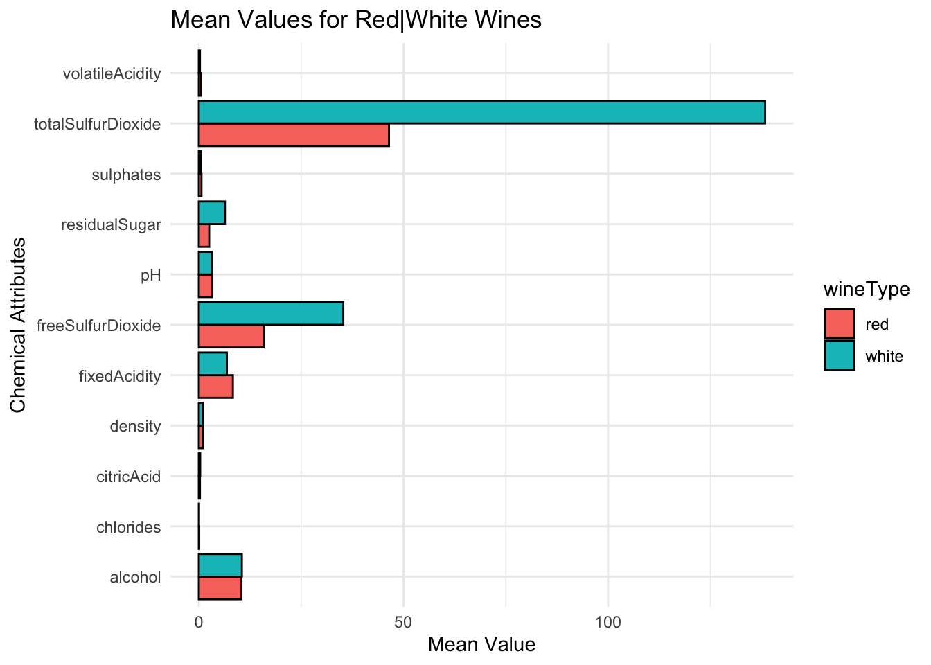
p2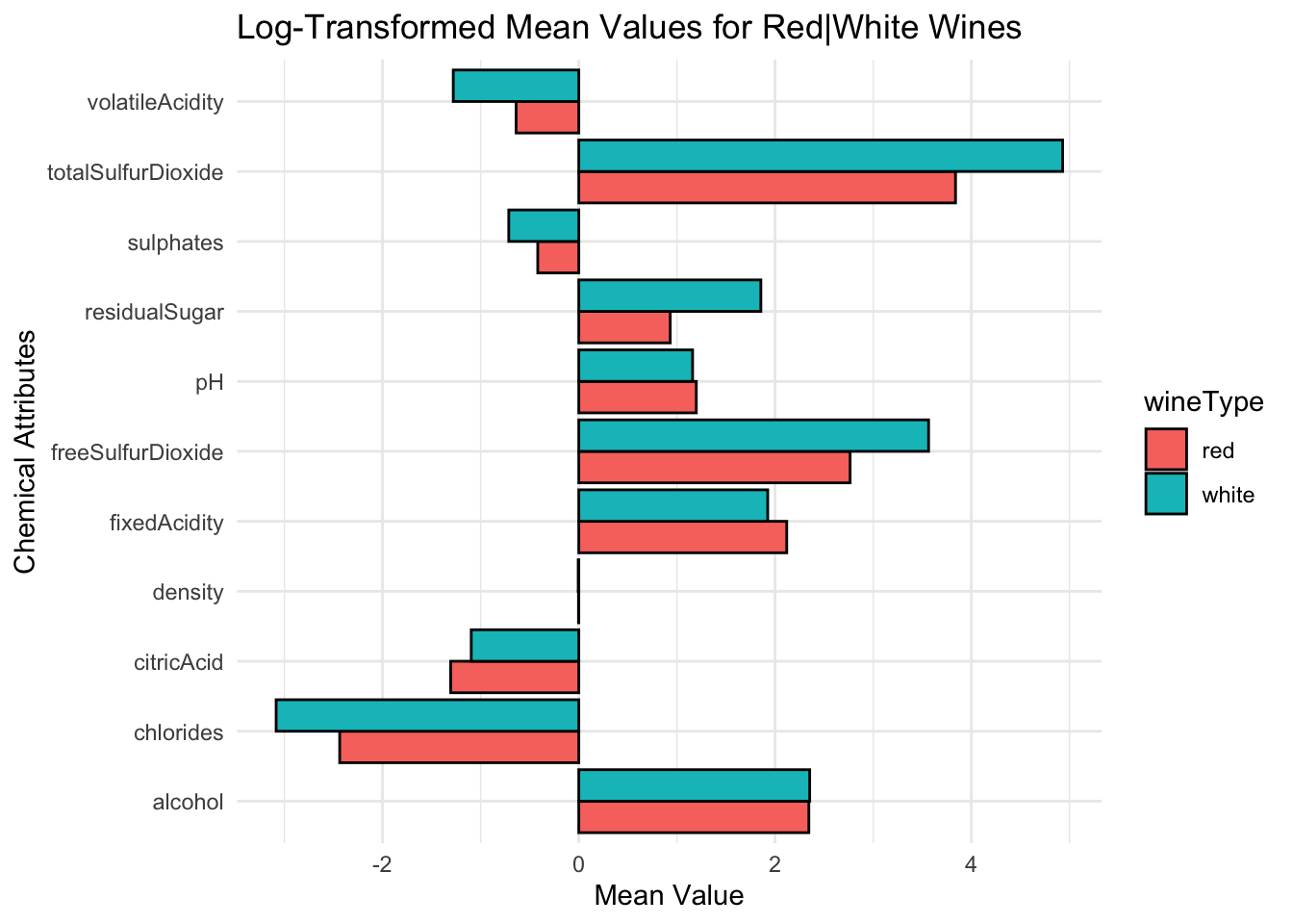
p3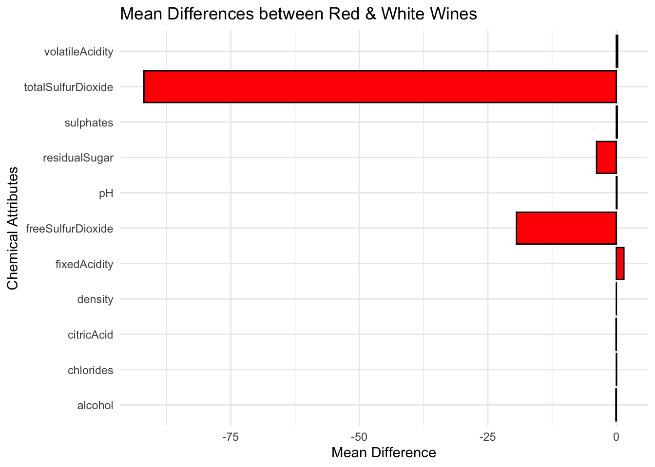
Perform MANOVA to determine if there are a significant difference in mean vectors between red and white wines with a 95% confidence level.
wineManova <- manova(cbind(chlorides, density, pH, sulphates,
                           alcohol, fixedAcidity, volatileAcidity,
                           citricAcid, residualSugar, freeSulfurDioxide,
                           totalSulfurDioxide) ~ wineType, data = wineDs)

# Print the summary of the MANOVA
summary(wineManova)
Df Pillai approx F num Df den Df Pr(>F)
wineType 1 0.86158 3669.6 11 6485 < 0.00000000000000022 ***
Residuals 6495
---
Signif. codes: 0 '***' 0.001 '**' 0.01 '*' 0.05 '.' 0.1 ' ' 1MANOVA Results
Perform Classification Modeling on Red & White Wines
Train-Test Split & Cross-Validation Set up
splitIndex <- createDataPartition(wineDs$wineType, p = 0.7, list = FALSE)
trainData <- wineDs[splitIndex, ]
testData <- wineDs[-splitIndex, ]

# Create Repeated cross-validation
ctrl <- trainControl(method = "repeatedcv",
                     number = 5,
                     repeats = 3,
                     verboseIter = FALSE)
Random Forest, SVM and Logistic Models
set.seed(2013)

# Train Random Forest
rfModel <- train(wineType ~ .,
                  data = trainData,
                  method = "rf",
                  control = ctrl,
                  ntree = 200)

# Train Logistic Regression
logisticModel <- train(wineType ~ .,
                       data = trainData,
                       method = "glm",
                       family = "binomial")

# Train Support Vector Machine
svmModel <- train(wineType ~ .,
                  data = trainData,
                  method = "svmRadial",
                  trControl = ctrl)

# Make predictions on the test set for each model
rfPred <- predict(rfModel, newdata = testData)
logisticPred <- predict(logisticModel, newdata = testData)
svmPred <- predict(svmModel, newdata = testData)
Metrics & Variable Importance
# Random Forest model metrics
confMatrixRF <- confusionMatrix(rfPred, testData$wineType,
                                dnn = c("Prediction", "Reference"))
accuracyRF <- confMatrixRF$overall["Accuracy"]

# Logistic Regression model metrics
confMatrixLogistic <- confusionMatrix(logisticPred, testData$wineType,
                                      dnn = c("Prediction", "Reference"))
accuracyLogistic <- confMatrixLogistic$overall["Accuracy"]

# SVM model metrics
confMatrixSVM <- confusionMatrix(svmPred, testData$wineType,
                                 dnn = c("Prediction", "Reference"))
accuracySVM <- confMatrixSVM$overall["Accuracy"]

# Plot Confusion Matrices
plotCM <- function(confMatrix, modelName) {
  plt <- as.data.frame(confMatrix$table)
  plt$Prediction <- factor(plt$Prediction,
                           levels = rev(levels(plt$Prediction)))

  ggplot(plt, aes(Prediction, Reference, fill = Freq)) +
    geom_tile() + geom_text(aes(label = Freq)) +
    scale_fill_gradient(low = "white", high = "#00859B") +
    labs(title = paste("Confusion Matrix -", modelName),
         x = "Reference", y = "Prediction") +
    scale_x_discrete(labels = levels(testData$wineType)) +
    scale_y_discrete(labels = levels(testData$wineType))
}

#confMatrixRF
confMatrixLogistic
Confusion Matrix and Statistics
Reference
Prediction red white
red 473 6
white 6 1463
Accuracy : 0.9938
95% CI : (0.9893, 0.9968)
No Information Rate : 0.7541
P-Value [Acc > NIR] : <0.0000000000000002
Kappa : 0.9834
Mcnemar's Test P-Value : 1
Sensitivity : 0.9875
Specificity : 0.9959
Pos Pred Value : 0.9875
Neg Pred Value : 0.9959
Prevalence : 0.2459
Detection Rate : 0.2428
Detection Prevalence : 0.2459
Balanced Accuracy : 0.9917
'Positive' Class : red
#confMatrixSVM

# Plot Confusion Matrices for each model
plotCM(confMatrixRF, "Random Forest")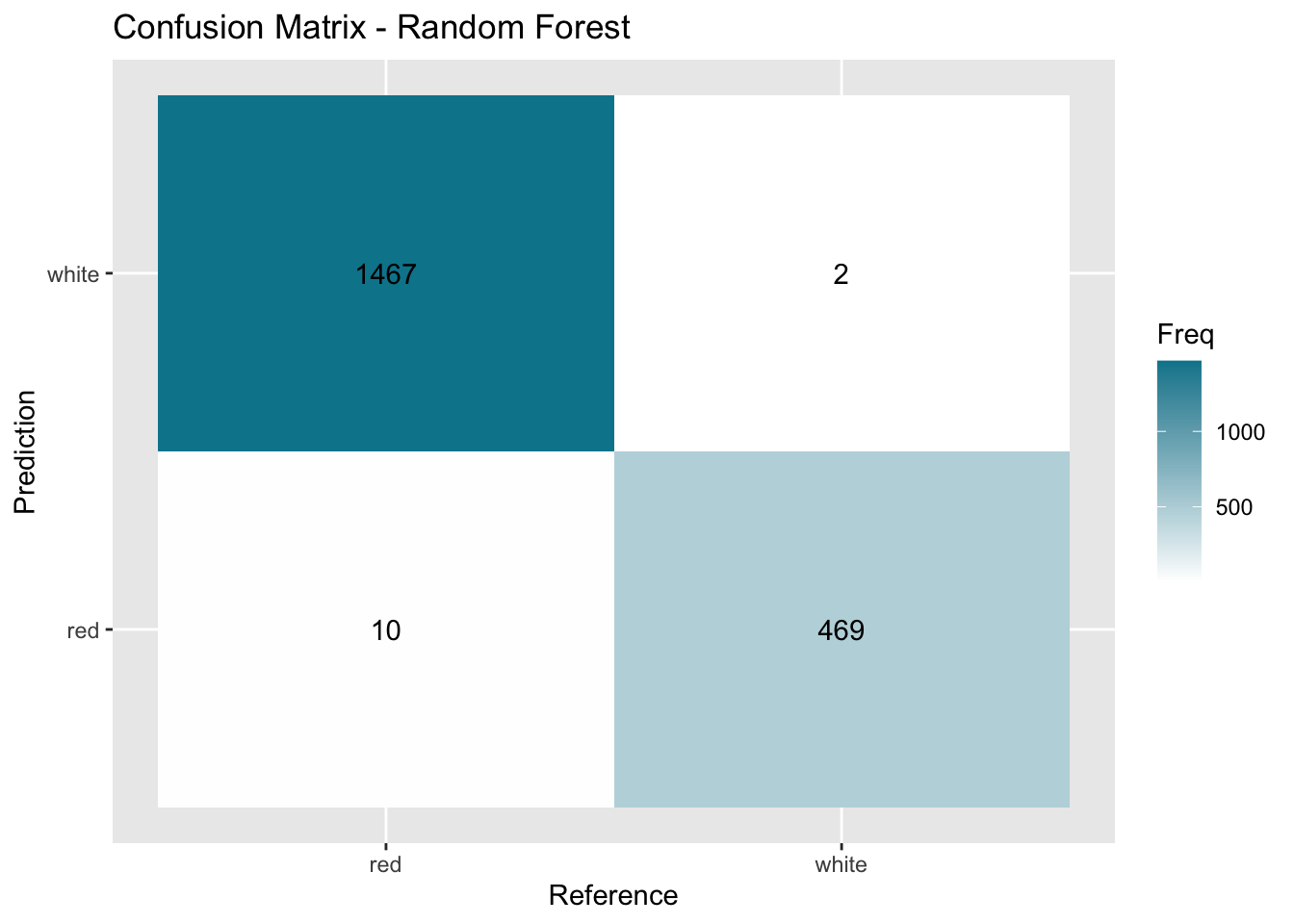
plotCM(confMatrixLogistic, "Logistic Regression")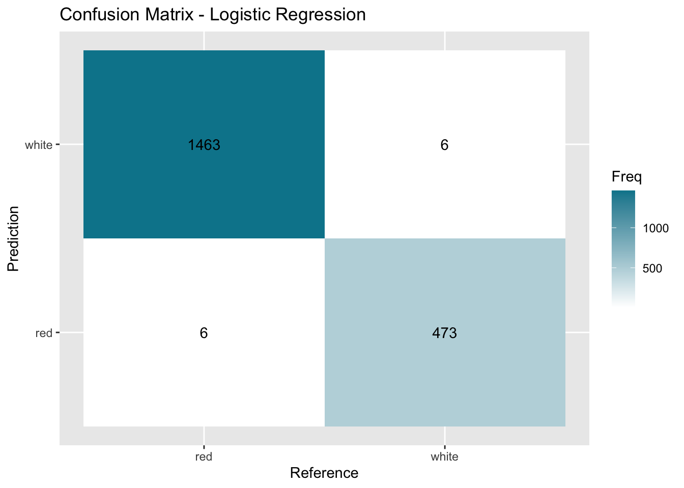
plotCM(confMatrixSVM, "Support Vector Machine (SVM)")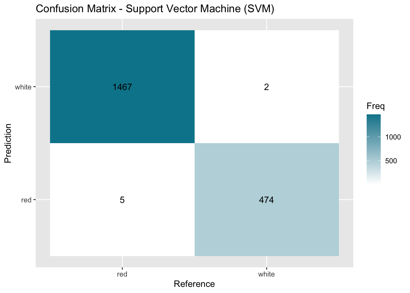
# Print the metrics for each model
print("Random Forest Model Results")
[1] "Random Forest Model Results"print(paste("Accuracy:", round(accuracyRF, 4)))[1] "Accuracy: 0.9938"print("Logistic Regression Model Results:")[1] "Logistic Regression Model Results:"print(paste("Accuracy:", round(accuracyLogistic, 4)))[1] "Accuracy: 0.9938"print("Support Vector Machine (SVM) Model Results:")[1] "Support Vector Machine (SVM) Model Results:"print(paste("Accuracy:", round(accuracySVM, 4)))[1] "Accuracy: 0.9964"# Get variable importance from the best model
varImp(rfModel)rf variable importance
Overall
chlorides 100.000
totalSulfurDioxide 80.296
volatileAcidity 43.041
freeSulfurDioxide 23.194
density 22.347
residualSugar 18.246
sulphates 17.811
fixedAcidity 12.766
citricAcid 4.859
pH 3.794
alcohol 0.000Classifying a New Red Wine Drawn From The Same Population
Clustering:
set.seed(123)

ds <- wineDs %>%
  select(-wineType)

ds <- scale(ds)

fviz_nbclust(ds, kmeans, method='silhouette')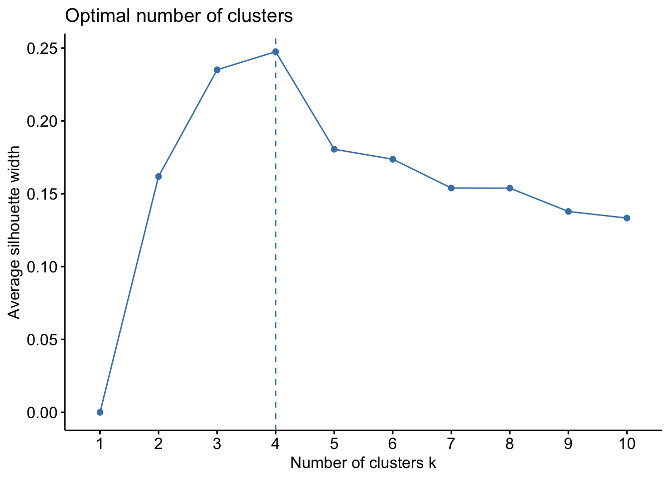
km.final <- kmeans(ds, 2, nstart = 30)

fviz_cluster(km.final, data = ds,
             geom = "point",
             ellipse.type = "convex",
             ggtheme = theme_bw())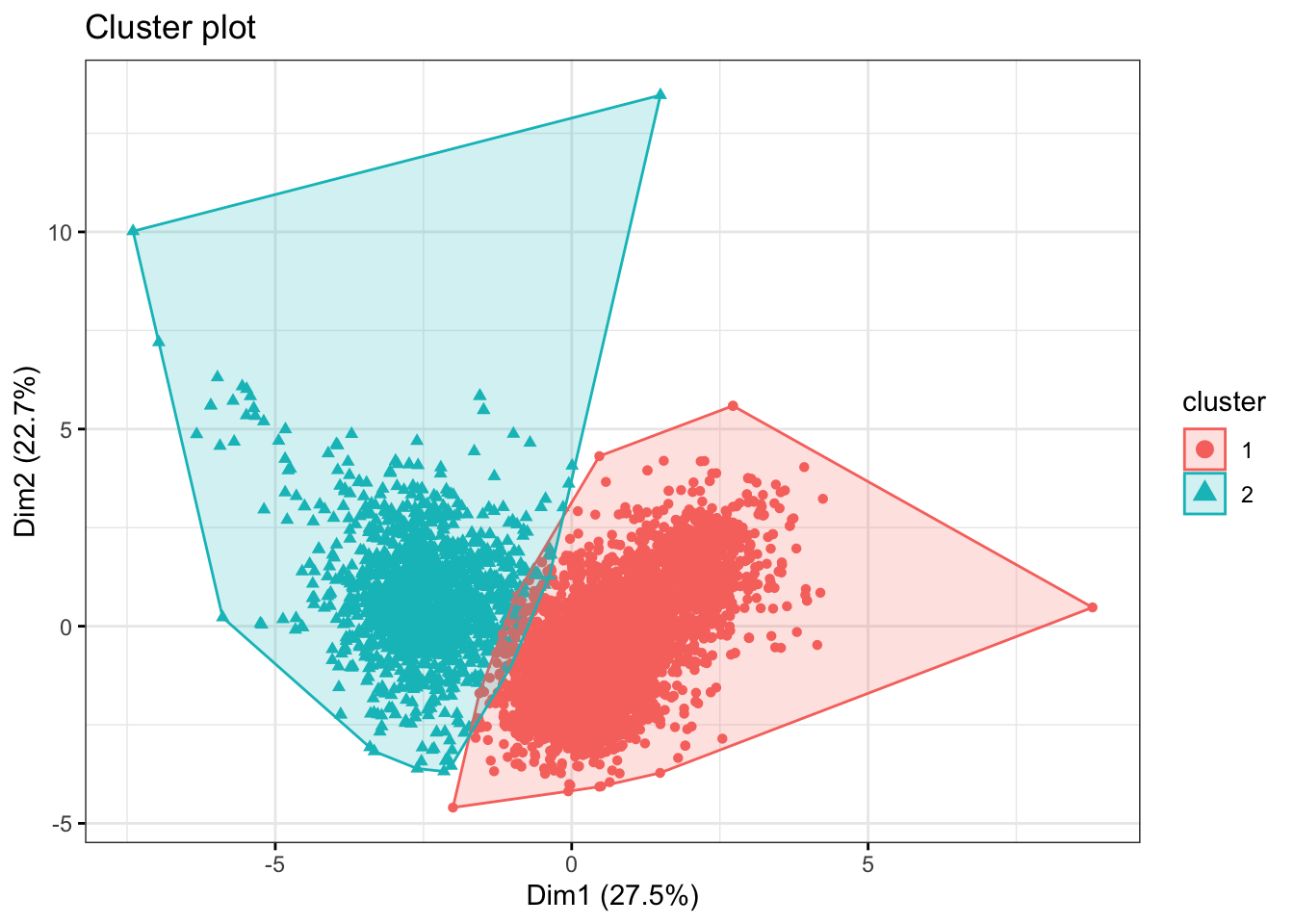
Goal 2: Which Variables Are The Most Important To Wine Quality In Red Wines.
Perform MANOVAs to determine if there are a significant difference in mean vectors between wines with different quality/quality groups with a 95% confidence level?
MANOVA for Quality Levels 3, 4, 5, 6, 7, 8
redWineDs <- wine %>%
  filter(wineType == "red") %>%
  select(-wineType)

# Extracting Columns
colVars <-  cbind(
  redWineDs$chlorides, redWineDs$density, redWineDs$pH, redWineDs$sulphates,
  redWineDs$alcohol, redWineDs$fixedAcidity, redWineDs$volatileAcidity,
  redWineDs$citricAcid, redWineDs$residualSugar, redWineDs$freeSulfurDioxide,
  redWineDs$totalSulfurDioxide
)

# MANOVA Analysis - Quality, levels = 3,4,5,6,7,8
manaovaTest <- manova(colVars ~ quality, data = redWineDs)
summary(manaovaTest)
Df Pillai approx F num Df den Df Pr(>F)
quality 1 0.36055 81.348 11 1587 < 0.00000000000000022 ***
Residuals 1597
---
Signif. codes: 0 '***' 0.001 '**' 0.01 '*' 0.05 '.' 0.1 ' ' 1MANOVA for Quality Groups [Low, Medium, High]
# Adding qualityGroup
redWineDs <- redWineDs %>%
  mutate(
    qualityGroup = case_when(
      quality %in% 3:4 ~ "Low",
      quality %in% 5:6 ~ "Medium",
      quality %in% 7:8 ~ "High"
    )
  ) %>%
  mutate(qualityGroup = factor(qualityGroup, levels = c("Low",
                                                        "Medium",
                                                        "High")))
colVarsCategorized <-  cbind(
  redWineDs$chlorides, redWineDs$density, redWineDs$pH,
  redWineDs$sulphates, redWineDs$alcohol, redWineDs$fixedAcidity,
  redWineDs$volatileAcidity, redWineDs$citricAcid,
  redWineDs$residualSugar, redWineDs$freeSulfurDioxide,
  redWineDs$totalSulfurDioxide
)

# MANOVA Analysis - QualityGroup, Levels = "Low", "Medium", "High"
manaovaTest <- manova(colVars ~ qualityGroup, data = redWineDs)
summary(manaovaTest)
Df Pillai approx F num Df den Df Pr(>F)
qualityGroup 2 0.30989 26.453 22 3174 < 0.00000000000000022 ***
Residuals 1596
---
Signif. codes: 0 '***' 0.001 '**' 0.01 '*' 0.05 '.' 0.1 ' ' 1Overall MANOVA Test Conclusion
Perform Classification on Quality for Red Wines
qualityDs <- redWineDs %>%
  mutate(quality = factor(quality, levels = c("3","4","5","6","7","8"))) %>%
  select(-qualityGroup)
# Split the dataset into training and testing sets
splitIndex <- createDataPartition(qualityDs$quality, p = 0.7, list = FALSE)
trainData <- qualityDs[splitIndex, ]
testData <- qualityDs[-splitIndex, ]
# Create a train control object for repeated cross-validation
ctrl <- trainControl(method = "repeatedcv",
number = 5,
repeats = 3,
verboseIter = FALSE)Random Forest and SVM models
set.seed(2013)
# Random Forest model
rfModel <- train(quality ~ .,
                  data = trainData,
                  method = "rf",
                  control = ctrl,
                  ntree = 200)

# (SVM) model
svmModel <- train(quality ~ .,
                  data = trainData,
                  method = "svmLinear",
                  trControl = ctrl)

# Make predictions on the test set for each model
rfPred <- predict(rfModel, newdata = testData)
svmPred <- predict(svmModel, newdata = testData)
Metrics & Variable Importance
# Random Forest confusion matrix
rfConfMatrix <- confusionMatrix(rfPred, testData$quality,
                                dnn = c("Prediction", "Reference"))
rfAccuracy <- rfConfMatrix$overall["Accuracy"]

# SVM confusion matrix
svmConfMatrix <- confusionMatrix(svmPred, testData$quality,
                                 dnn = c("Prediction", "Reference"))
svmAccuracy <- svmConfMatrix$overall["Accuracy"]

# Print the results
print(paste("Random Forest Accuracy:", rfAccuracy))
[1] "Random Forest Accuracy: 0.691823899371069"print(paste("SVM Accuracy:", svmAccuracy))[1] "SVM Accuracy: 0.59538784067086"rfConfMatrixConfusion Matrix and Statistics
Reference
Prediction 3 4 5 6 7 8
3 0 0 0 0 0 0
4 0 0 0 1 0 0
5 3 10 163 46 5 0
6 0 4 40 137 24 4
7 0 1 1 7 30 1
8 0 0 0 0 0 0
Overall Statistics
Accuracy : 0.6918
95% CI : (0.6482, 0.733)
No Information Rate : 0.4277
P-Value [Acc > NIR] : < 0.00000000000000022
Kappa : 0.4953
Mcnemar's Test P-Value : NA
Statistics by Class:
Class: 3 Class: 4 Class: 5 Class: 6 Class: 7 Class: 8
Sensitivity 0.000000 0.000000 0.7990 0.7173 0.50847 0.00000
Specificity 1.000000 0.997835 0.7656 0.7483 0.97608 1.00000
Pos Pred Value NaN 0.000000 0.7181 0.6555 0.75000 NaN
Neg Pred Value 0.993711 0.968487 0.8360 0.7985 0.93364 0.98952
Prevalence 0.006289 0.031447 0.4277 0.4004 0.12369 0.01048
Detection Rate 0.000000 0.000000 0.3417 0.2872 0.06289 0.00000
Detection Prevalence 0.000000 0.002096 0.4759 0.4382 0.08386 0.00000
Balanced Accuracy 0.500000 0.498918 0.7823 0.7328 0.74228 0.50000svmConfMatrixConfusion Matrix and Statistics
Reference
Prediction 3 4 5 6 7 8
3 0 0 1 0 0 0
4 0 0 0 0 0 0
5 2 11 159 66 6 0
6 1 4 44 125 53 5
7 0 0 0 0 0 0
8 0 0 0 0 0 0
Overall Statistics
Accuracy : 0.5954
95% CI : (0.5498, 0.6398)
No Information Rate : 0.4277
P-Value [Acc > NIR] : 0.0000000000001356
Kappa : 0.3101
Mcnemar's Test P-Value : NA
Statistics by Class:
Class: 3 Class: 4 Class: 5 Class: 6 Class: 7 Class: 8
Sensitivity 0.000000 0.00000 0.7794 0.6545 0.0000 0.00000
Specificity 0.997890 1.00000 0.6886 0.6259 1.0000 1.00000
Pos Pred Value 0.000000 NaN 0.6516 0.5388 NaN NaN
Neg Pred Value 0.993697 0.96855 0.8069 0.7306 0.8763 0.98952
Prevalence 0.006289 0.03145 0.4277 0.4004 0.1237 0.01048
Detection Rate 0.000000 0.00000 0.3333 0.2621 0.0000 0.00000
Detection Prevalence 0.002096 0.00000 0.5115 0.4864 0.0000 0.00000
Balanced Accuracy 0.498945 0.50000 0.7340 0.6402 0.5000 0.50000# Plot Confusion Matrices
plotCM <- function(confMatrix, modelName) {
plt <- as.data.frame(confMatrix$table)
plt$Prediction <- factor(plt$Prediction,
levels = rev(levels(plt$Prediction)))
ggplot(plt, aes(Prediction, Reference, fill = Freq)) +
geom_tile() + geom_text(aes(label = Freq)) +
scale_fill_gradient(low = "white", high = "#00859B") +
labs(title = paste("Confusion Matrix -", modelName),
x = "Reference", y = "Prediction") +
scale_x_discrete(labels = levels(testData$quality)) +
scale_y_discrete(labels = levels(testData$quality))
}
plotCM(rfConfMatrix, "Random Forest")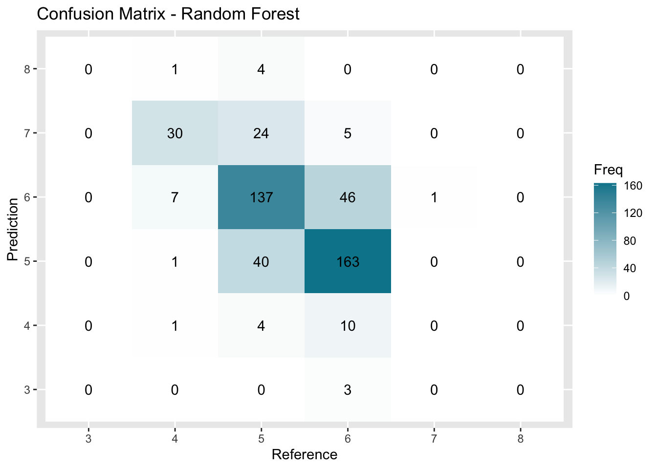
plotCM(svmConfMatrix, "SVM")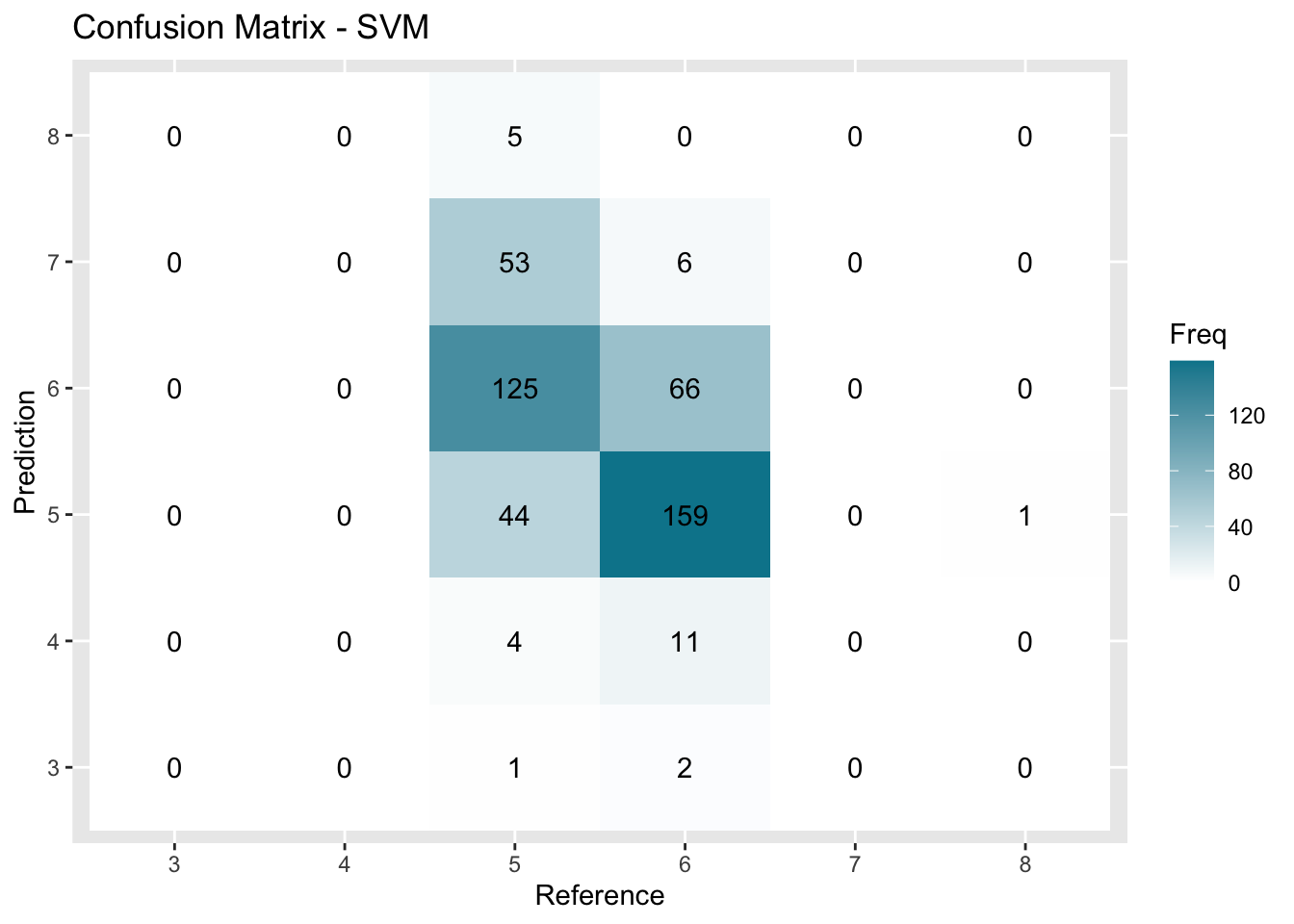
plot(varImp(rfModel))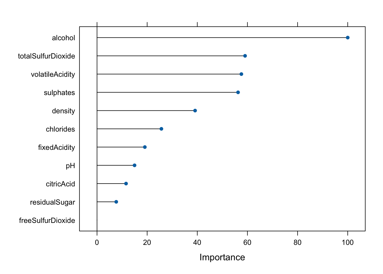
Perform Principal Component Analysis
Part 1
ds <- select(qualityDs, -quality)

# Perform PCA
pcaResults <- prcomp(ds, scale = T, center = T)

# Print PCA summary
summary(pcaResults)
Importance of components:
PC1 PC2 PC3 PC4 PC5 PC6 PC7
Standard deviation 1.7604 1.3878 1.2452 1.1015 0.97943 0.81216 0.76406
Proportion of Variance 0.2817 0.1751 0.1410 0.1103 0.08721 0.05996 0.05307
Cumulative Proportion 0.2817 0.4568 0.5978 0.7081 0.79528 0.85525 0.90832
PC8 PC9 PC10 PC11
Standard deviation 0.65035 0.58706 0.42583 0.24405
Proportion of Variance 0.03845 0.03133 0.01648 0.00541
Cumulative Proportion 0.94677 0.97810 0.99459 1.00000# Visualize PCA results
fviz_eig(pcaResults, addlabels = TRUE, kaiser = TRUE)
fviz_pca_ind(pcaResults, geom = "point", col.ind = qualityDs$quality, palette = "jco")
fviz_pca_biplot(pcaResults, geom = "arrow", col.var = "contrib", palette = "jco", alpha = 0.7)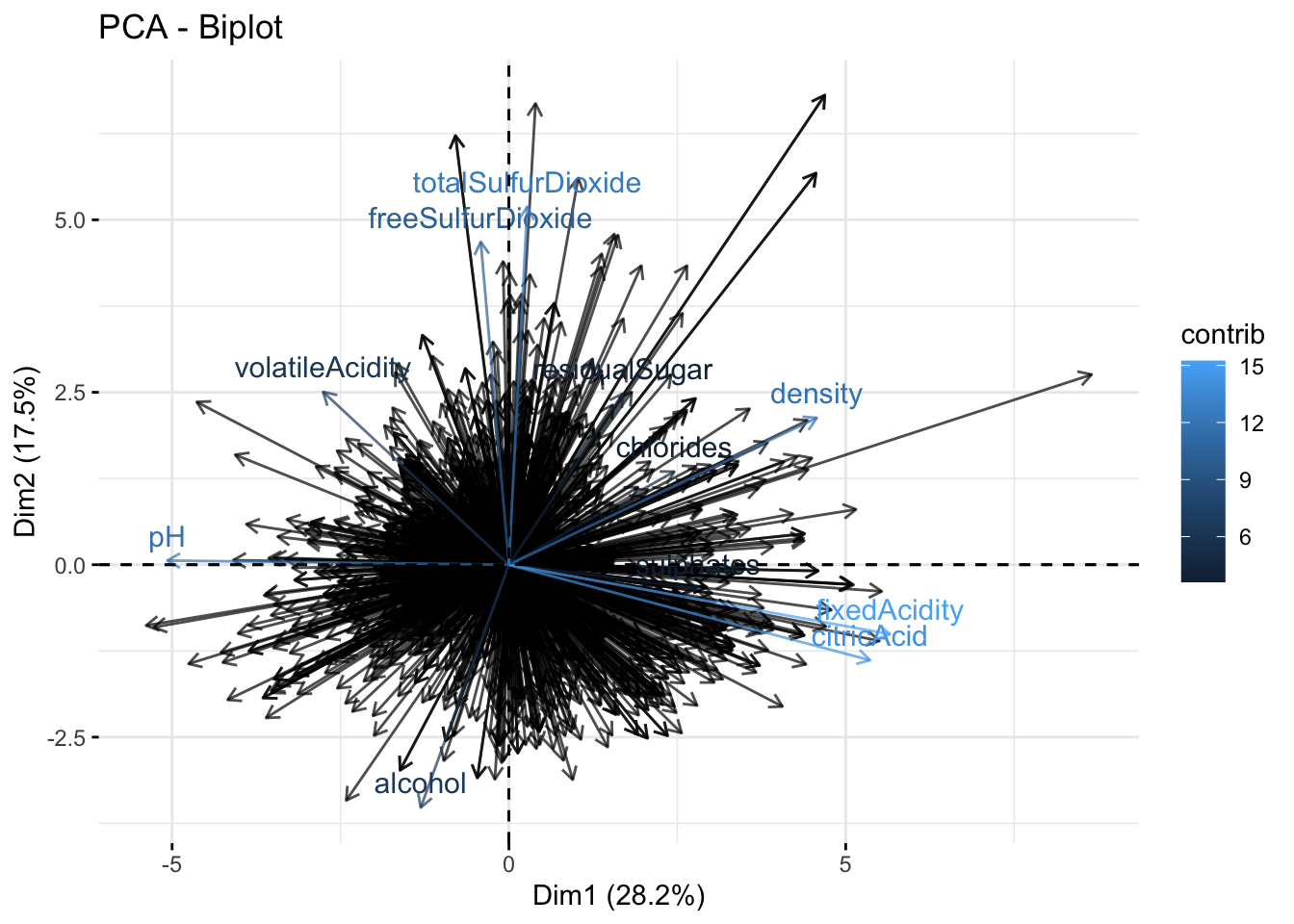
pcaDs <- rownames_to_column(as.data.frame(pcaResults$rotation))

pcaDs %>%
  select(rowname, PC1, PC2)
rowname PC1 PC2
1 chlorides 0.21224658 0.148051555
2 density 0.39535301 0.233575490
3 pH -0.43851962 0.006710793
4 sulphates 0.24292133 -0.037553916
5 alcohol -0.11323207 -0.386180959
6 fixedAcidity 0.48931422 -0.110502738
7 volatileAcidity -0.23858436 0.274930480
8 citricAcid 0.46363166 -0.151791356
9 residualSugar 0.14610715 0.272080238
10 freeSulfurDioxide -0.03615752 0.513566812
11 totalSulfurDioxide 0.02357485 0.569486959# Adding back the quality with principal components
prc <- select(qualityDs, quality) %>%
bind_cols(as.data.frame(pcaResults$x)) %>%
select(quality, PC1, PC2)
# Rename columns
prc <- prc %>%
rename(
"Quality" = quality,
"Wine Body" = PC1,
"Fermentation Characteristics" = PC2
)
prc2 <- select(qualityDs, quality) %>%
bind_cols(as.data.frame(pcaResults$x)) %>%
select(quality, PC1, PC2, PC3, PC4, PC5, PC6, PC7, PC8, PC9, PC10, PC11)
prc2 <- prc2 %>%
rename("Quality" = quality)
prc2# A tibble: 1,599 × 12
Quality PC1 PC2 PC3 PC4 PC5 PC6 PC7 PC8 PC9
<fct> <dbl> <dbl> <dbl> <dbl> <dbl> <dbl> <dbl> <dbl> <dbl>
1 5 -1.62 0.451 -1.77 0.0437 -0.0670 -0.914 0.161 0.282 -0.00510
2 5 -0.799 1.86 -0.911 0.548 0.0184 0.929 1.01 -0.762 0.521
3 5 -0.748 0.882 -1.17 0.411 0.0435 0.401 0.539 -0.598 0.0868
4 6 2.36 -0.270 0.243 -0.928 1.50 -0.131 -0.344 0.455 -0.0915
5 5 -1.62 0.451 -1.77 0.0437 -0.0670 -0.914 0.161 0.282 -0.00510
6 5 -1.58 0.569 -1.54 0.0237 0.110 -0.993 0.110 0.314 0.0343
7 5 -1.10 0.608 -1.08 -0.344 1.13 0.175 -0.261 -0.240 0.0273
8 7 -2.25 -0.417 -0.987 -0.00120 0.780 0.286 -0.131 -0.119 0.614
9 7 -1.09 -0.308 -1.52 0.00331 0.227 -0.512 -0.250 -0.439 0.399
10 5 0.655 1.66 1.21 -0.824 -1.72 -0.476 -0.230 -0.839 -1.27
# ℹ 1,589 more rows
# ℹ 2 more variables: PC10 <dbl>, PC11 <dbl>Part 2
set.seed(2013)

splitIndex <- createDataPartition(prc$Quality, p = 0.7, list = FALSE)
trainData <- prc[splitIndex, ]
testData <- prc[-splitIndex, ]

# Create Repeated cross-validation
ctrl <- trainControl(method = "repeatedcv",
                     number = 5,
                     repeats = 3,
                     verboseIter = FALSE)

# Train Random Forest
rfModel <- train(Quality ~ .,
                  data = trainData,
                  method = "rf",
                  control = ctrl,
                  ntree = 200)
note: only 1 unique complexity parameters in default grid. Truncating the grid to 1 .# Make predictions on the test set for each model
rfPred <- predict(rfModel, newdata = testData)
# Plot Confusion Matrices
plotCM <- function(confMatrix, modelName) {
plt <- as.data.frame(confMatrix$table)
plt$Prediction <- factor(plt$Prediction,
levels = rev(levels(plt$Prediction)))
ggplot(plt, aes(Prediction, Reference, fill = Freq)) +
geom_tile() + geom_text(aes(label = Freq)) +
scale_fill_gradient(low = "white", high = "#00859B") +
labs(title = paste("Confusion Matrix -", modelName),
x = "Reference", y = "Prediction") +
scale_x_discrete(labels = levels(testData$Quality)) +
scale_y_discrete(labels = levels(testData$Quality))
}
# Random Forest metrics
rfConfMatrix <- confusionMatrix(rfPred, testData$Quality,
dnn = c("Prediction", "Reference"))
rfAccuracy <- rfConfMatrix$overall["Accuracy"]
print(paste("Random Forest Accuracy:", rfAccuracy))[1] "Random Forest Accuracy: 0.580712788259958"plotCM(rfConfMatrix, "Random Forest")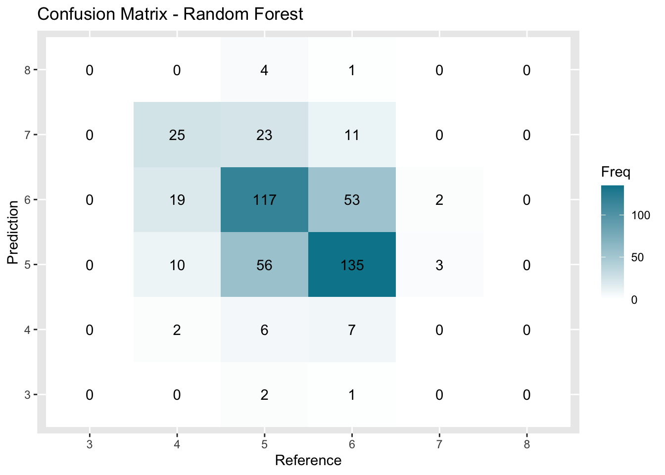
rfConfMatrix$table Reference
Prediction 3 4 5 6 7 8
3 0 0 0 0 0 0
4 0 0 3 2 0 0
5 1 7 135 53 11 1
6 2 6 56 117 23 4
7 0 2 10 19 25 0
8 0 0 0 0 0 0# Variable Importance
varImp(rfModel)rf variable importance
Overall
`Fermentation Characteristics` 100
`Wine Body` 0set.seed(2013)
splitIndex <- createDataPartition(prc2$Quality, p = 0.7, list = FALSE)
trainData <- prc2[splitIndex, ]
testData <- prc2[-splitIndex, ]
# Create Repeated cross-validation
ctrl <- trainControl(method = "repeatedcv",
number = 5,
repeats = 3,
verboseIter = FALSE)
# Train Random Forest
rfModel <- train(Quality ~ .,
data = trainData,
method = "rf",
control = ctrl,
ntree = 200)
# Make predictions on the test set for each model
rfPred <- predict(rfModel, newdata = testData)


# Plot Confusion Matrices
plotCM <- function(confMatrix, modelName) {
  plt <- as.data.frame(confMatrix$table)
  plt$Prediction <- factor(plt$Prediction,
                           levels = rev(levels(plt$Prediction)))

  ggplot(plt, aes(Prediction, Reference, fill = Freq)) +
    geom_tile() + geom_text(aes(label = Freq)) +
    scale_fill_gradient(low = "white", high = "#00859B") +
    labs(title = paste("Confusion Matrix -", modelName),
         x = "Reference", y = "Prediction") +
    scale_x_discrete(labels = levels(testData$Quality)) +
    scale_y_discrete(labels = levels(testData$Quality))
}

# Random Forest metrics
rfConfMatrix <- confusionMatrix(rfPred, testData$Quality,
                                dnn = c("Prediction", "Reference"))
rfAccuracy <- rfConfMatrix$overall["Accuracy"]
print(paste("Random Forest Accuracy:", rfAccuracy))
[1] "Random Forest Accuracy: 0.681341719077568"plotCM(rfConfMatrix, "Random Forest")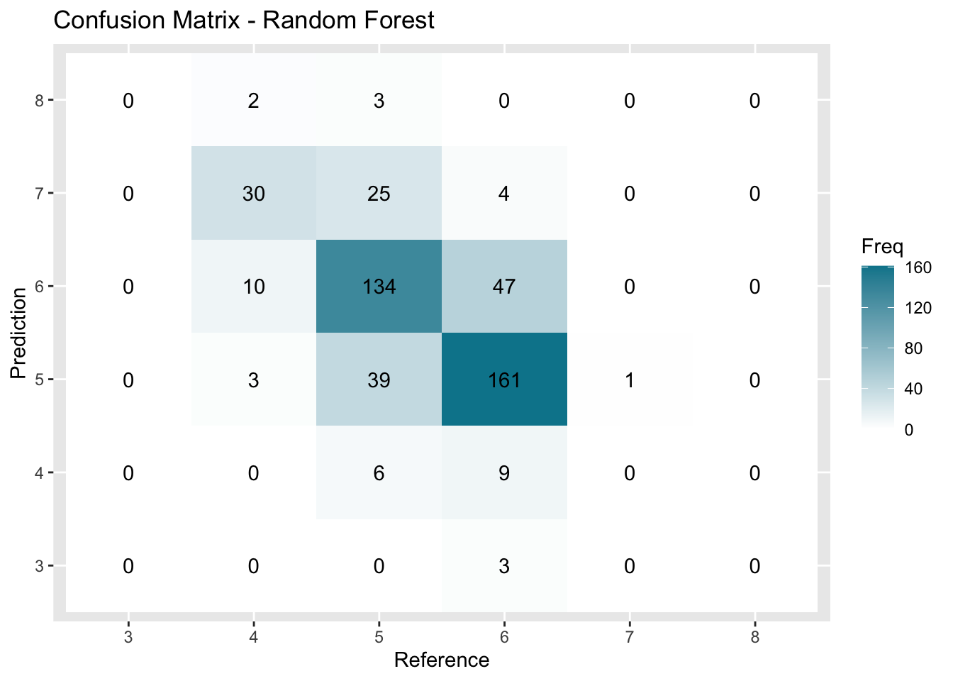
rfConfMatrixConfusion Matrix and Statistics
Reference
Prediction 3 4 5 6 7 8
3 0 0 0 0 0 0
4 0 0 1 0 0 0
5 3 9 161 47 4 0
6 0 6 39 134 25 3
7 0 0 3 10 30 2
8 0 0 0 0 0 0
Overall Statistics
Accuracy : 0.6813
95% CI : (0.6374, 0.723)
No Information Rate : 0.4277
P-Value [Acc > NIR] : < 0.00000000000000022
Kappa : 0.4807
Mcnemar's Test P-Value : NA
Statistics by Class:
Class: 3 Class: 4 Class: 5 Class: 6 Class: 7 Class: 8
Sensitivity 0.000000 0.000000 0.7892 0.7016 0.50847 0.00000
Specificity 1.000000 0.997835 0.7692 0.7448 0.96411 1.00000
Pos Pred Value NaN 0.000000 0.7188 0.6473 0.66667 NaN
Neg Pred Value 0.993711 0.968487 0.8300 0.7889 0.93287 0.98952
Prevalence 0.006289 0.031447 0.4277 0.4004 0.12369 0.01048
Detection Rate 0.000000 0.000000 0.3375 0.2809 0.06289 0.00000
Detection Prevalence 0.000000 0.002096 0.4696 0.4340 0.09434 0.00000
Balanced Accuracy 0.500000 0.498918 0.7792 0.7232 0.73629 0.50000# Variable Importance
varImp(rfModel)rf variable importance
Overall
PC2 100.000
PC3 80.491
PC5 32.468
PC9 30.188
PC1 16.023
PC4 7.563
PC7 6.410
PC8 5.631
PC11 3.630
PC10 3.489
PC6 0.000Repeat for Grouped Quality Setting (Low, Medium, High)
Setting up data for classification
groupedQualityDs <- redWineDs %>%
  select(-quality)
Train-Test-Split & Cross-Validation Set up
# Split the dataset into training and testing sets
splitIndex <- createDataPartition(groupedQualityDs$qualityGroup, p = 0.7, list = FALSE)
trainData <- groupedQualityDs[splitIndex, ]
testData <- groupedQualityDs[-splitIndex, ]

# Create a train control object for repeated cross-validation
ctrl <- trainControl(method = "repeatedcv",
                     number = 5,
                     repeats = 3,
                     verboseIter = FALSE)
Random Forest and SVM models
set.seed(2013)
# Train Random Forest classifier using caret
rfModel <- train(qualityGroup ~ .,
                  data = trainData,
                  method = "rf",
                  control = ctrl,
                  ntree = 200)

# Train Support Vector Machine (SVM) model using caret
svmModel <- train(qualityGroup ~ .,
                  data = trainData,
                  method = "svmRadial",
                  trControl = ctrl)

# Make predictions on the test set for each model
rfPred <- predict(rfModel, newdata = testData)
svmPred <- predict(svmModel, newdata = testData)
Metrics
# Plot Confusion Matrices
plotCM <- function(confMatrix, modelName) {
  plt <- as.data.frame(confMatrix$table)
  plt$Prediction <- factor(plt$Prediction,
                           levels = rev(levels(plt$Prediction)))

  ggplot(plt, aes(Prediction, Reference, fill = Freq)) +
    geom_tile() + geom_text(aes(label = Freq)) +
    scale_fill_gradient(low = "white", high = "#00859B") +
    labs(title = paste("Confusion Matrix -", modelName),
         x = "Reference", y = "Prediction") +
    scale_x_discrete(labels = levels(testData$qualityGroup)) +
    scale_y_discrete(labels = levels(testData$qualityGroup))
}

# Random Forest metrics
rfConfMatrix <- confusionMatrix(rfPred, testData$qualityGroup,
                                dnn = c("Prediction", "Reference"))
svmConfMatrix <- confusionMatrix(svmPred, testData$qualityGroup,
                                 dnn = c("Prediction", "Reference"))

rfConfMatrix
Confusion Matrix and Statistics
Reference
Prediction Low Medium High
Low 0 0 0
Medium 18 388 39
High 0 7 26
Overall Statistics
Accuracy : 0.8661
95% CI : (0.8323, 0.8953)
No Information Rate : 0.8264
P-Value [Acc > NIR] : 0.01092
Kappa : 0.395
Mcnemar's Test P-Value : NA
Statistics by Class:
Class: Low Class: Medium Class: High
Sensitivity 0.00000 0.9823 0.40000
Specificity 1.00000 0.3133 0.98305
Pos Pred Value NaN 0.8719 0.78788
Neg Pred Value 0.96234 0.7879 0.91236
Prevalence 0.03766 0.8264 0.13598
Detection Rate 0.00000 0.8117 0.05439
Detection Prevalence 0.00000 0.9310 0.06904
Balanced Accuracy 0.50000 0.6478 0.69153svmConfMatrixConfusion Matrix and Statistics
Reference
Prediction Low Medium High
Low 0 0 0
Medium 18 393 50
High 0 2 15
Overall Statistics
Accuracy : 0.8536
95% CI : (0.8186, 0.884)
No Information Rate : 0.8264
P-Value [Acc > NIR] : 0.06328
Kappa : 0.2611
Mcnemar's Test P-Value : NA
Statistics by Class:
Class: Low Class: Medium Class: High
Sensitivity 0.00000 0.9949 0.23077
Specificity 1.00000 0.1807 0.99516
Pos Pred Value NaN 0.8525 0.88235
Neg Pred Value 0.96234 0.8824 0.89154
Prevalence 0.03766 0.8264 0.13598
Detection Rate 0.00000 0.8222 0.03138
Detection Prevalence 0.00000 0.9644 0.03556
Balanced Accuracy 0.50000 0.5878 0.61296plotCM(rfConfMatrix, "Random Forest")
plotCM(svmConfMatrix, "SVM")
Look at variable importance
plot(varImp(rfModel))